Hello World (Jupyter)

Depending on you Python installation and configuration you may have pip3 instead of pip available in your terminal. If you do have pip3 replace pip with pip3 in your command, i.e., pip3 install kaskada

You can see what version of Python pip uses by running pip -V

Installing kaskada for the first time can take 10-15 minutes while some external dependencies are built. Subsequent installs and upgrades are generally faster.

⭢ Read more about installing Kaskada in Locally

Now that we have everything installed let’s fire up a notebook and get the remaining components of Kaskada installed.

Using a terminal start a new Jupyter notebook using the command

Start a Jupyter notebook.

jupyter notebook

The jupyter command should activate your browser and you can open a new notebook. Create a new code cell in your new notebook and enter the following code in the code cell.

from kaskada.api.session import LocalBuilder

session = LocalBuilder().build()

Run this cell inside your notebook and you should see some output similar to the following

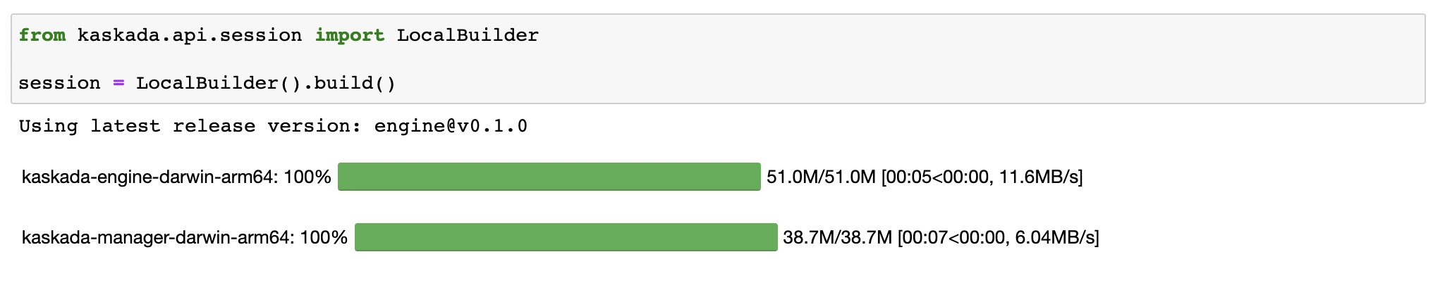
Sample output of Kaskada installation within a Jupyter notebook

Figure 1. Sample output of Kaskada’s installation within a Jupyter notebook.

This command imports the client’s LocalBuilder and uses this builder to create a session. This is the first time we are running the builder on this machine. The builder will download (if needed) the latest release of Kaskada’s components from GitHub and then run these components on your local machine. The command will generate some output during the download, install and run process.

⭢ Read more about connecting to Kaskada in Installing

Auto Recovery

Built into the local session, there are health check watchers that monitor the status of local services in case of failure or unavailability. If the services fail or are no longer available, the local session will attempt to automatically recover from failure. To disable this feature, use the keep_alive(False) builder argument.

from kaskada.api.session import LocalBuilder

session = LocalBuilder().keep_alive(False).build()

Let’s now create a small table and write a simple query to see that everything is working correctly with our setup.

Enable the Kaskada magic command

Kaskada’s client includes notebook customizations that allow us to write queries in the Fenl language but also receive and render the results of our queries in our notebooks. We need to enable these customizations first before we can use them.

So in a new code cell input the following command and run this cell.

Enable fenlmagic in this notebook

%load_ext fenlmagic

Now we can start a code cell in our notebook with the first line being the string %%fenl to indicate that this cell will contain code in the Fenl language. The special string %%fenl will also connect to the Kaskada components that we installed that will execute the query and report back any results to our notebook.

Congratulations, you now have Kaskada locally installed and you can start loading and querying your data using Kaskada inside a Jupyter notebook.

Loading Data into a Table

Kaskada stores data in tables. Tables consist of multiple rows, and each row is a value of the same type. When querying Kaskada, the contents of a table are interpreted as a discrete timeline: the value associated with each event corresponds to a value in the timeline.

Creating a Table

Every table is associated with a schema which defines the structure of each event in the table. Schemas are inferred from the data you load into a table, however, some columns are required by Kaskada’s data model. Every table must include a column identifying the time and entity associated with each row.

When creating a table, you must tell Kaskada which columns contain the time and entity of each row:

The time column is specified using the time_column_name parameter. This parameter must identify a column name in the table’s data which contains time values. The time should refer to when the event occurred.
The entity key is specified using the entity_key_column_name parameter. This parameter must identify a column name in the table’s data which contains the entity key value. The entity key should identify a thing in the world that each event is associated with. Don’t worry too much about picking the "right" value - it’s easy to change the entity using the with_key() function.

⭢ Read more about configuring tables in Tables

⭢ Read more about the expected structure of input files in Expected File Format

from kaskada import table
from kaskada.api.session import LocalBuilder

session = LocalBuilder().build()

table.create_table(
  # The table's name
  table_name = "Purchase",
  # The name of a column in your data that contains the time associated with each row
  time_column_name = "purchase_time",
  # The name of a column in your data that contains the entity key associated with each row
  entity_key_column_name = "customer_id",
)

Show result

The response from the create_table is a table object with contents similar to:

table {
  table_id: "76b***2e5"
  table_name: "Purchase"
  time_column_name: "purchase_time"
  entity_key_column_name: "customer_id"
  subsort_column_name: "subsort_id"
  create_time {
    seconds: 1634250064
    nanos: 422017488
  }
  update_time {
    seconds: 1634250064
    nanos: 422017488
  }
}
request_details {
  request_id: "fe6bed41fa29cea6ca85fe20bea6ef4a"
}

This creates a table named Purchase. Any data loaded into this table must have a timestamp field named purchase_time, a field named customer_id, and a field named subsort_id.

Idiomatic Kaskada

We like to use CamelCase to name tables because it helps distinguish data sources from transformed values and function names.

Loading data

Now that we’ve created a table, we’re ready to load some data into it.

A table must be created before data can be loaded into it.

Data can be loaded into a table in multiple ways. In this example we’ll load the contents of a Parquet file into the table.

⭢ Read more about the different ways to load data in Loading Data

from kaskada import table
from kaskada.api.session import LocalBuilder

session = LocalBuilder().build()

# A sample Parquet file provided by Kaskada for testing
# Available at https://drive.google.com/uc?export=download&id=1SLdIw9uc0RGHY-eKzS30UBhN0NJtslkk
purchases_path = "/absolute/path/to/purchases.parquet"

# Upload the files's contents to the Purchase table (which was created in the previous step)
table.load(table_name = "Purchase", file = purchases_path)

Show result

The result of running load is a data_token_id. The data token ID is a unique reference to the data currently stored in the system. Data tokens enable repeatable queries: queries performed against the same data token always run on the same input data.

data_token_id: "aa2***a6b9"
request_details {
  request_id: "fe6bed41fa29cea6ca85fe20bea6ef4b"
}

The file’s content is added to the table.

Querying Data

Enabling the Kaskada "magic" command

So in a new code cell input the following command and run this cell.

Enable fenlmagic in this notebook

%load_ext fenlmagic

Writing Queries

You can make Fenl queries by prefixing a query block with %%fenl. The query results will be computed and returned as a Pandas dataframe. The query content starts on the next line and includes the rest of the code block’s contents.

Let’s start by looking at the Purchase table without any filters, this query will return all of the columns and rows contained in a table:

%%fenl
Purchase

This query will return all of the columns and rows contained in a table. It can be helpful to limit your results to a single entity. This makes it easier to see how a single entity changes over time.

%%fenl
Purchase | when(Purchase.customer_id == "patrick")

In this example, we build a pipeline of functions using the | character. We begin with the timeline produced by the table Purchase, then filter it to the set of times where the purchase’s customer is "patrick" using the when() function.

Kaskada’s query language provides a rich set of operations for reasoning about time. Here’s a more sophisticated example that touches on many of the unique features of Kaskada queries:

%%fenl
# How many big purchases happen each hour and where?
# Anything can be named and re-used
let hourly_big_purchases = Purchase
| when(Purchase.amount > 10)

# Filter anywhere
| count(window=since(hourly()))

# Aggregate anything
| when(hourly())

# Shift timelines relative to each other
let purchases_now = count(Purchase)
let purchases_yesterday =
   purchases_now | shift_by(days(1))

# Records are just another type
in { hourly_big_purchases, purchases_in_last_day: purchases_now - purchases_yesterday }

⭢ Read more about writing queries in Queries

Configuring query execution

A given query can be computed in different ways. You can configure how a query is executed by providing flags to the %%fenl block.

Changing how the result timeline is output

When you make a query, the resulting timeline is interpreted in one of two ways: as a history or as a snapshot.

A timeline History generates a value each time the timeline changes, and each row is associated with a different entity and point in time.
A timeline Snapshot generates a value for each entity at the same point in time; each row is associated with a different entity, but all rows are associated with the same time.

By default, timelines are output as histories. You can output a timeline as a snapshot by setting the --result-behavior fenlmagic argument to final-results.

%%fenl --result-behavior final-results
Purchase | when(Purchase.customer_id == "patrick")

Limiting how many rows are returned

You can limit the number of rows returned from a query:

%%fenl --preview-rows 10
Purchase | when(Purchase.customer_id == "patrick")

This may return more rows that you asked for. Kaskada computes data in batches. When you configure --preview-rows Kaskada stops processing at the end of a batch once the given number of rows have been computed, and returns all the rows that were computed.

Assigning results to a variable

To capture the result of a query and assign it to the variable query_result:

%%fenl --var query_result
Purchase | when(Purchase.customer_id == "patrick")

You can now inspect the resulting dataframe, or the original query string:

# The result dataframe
query_result.dataframe

# The original query expression
query_result.expression

⭢ Read more about configuring queries in Configuring Queries

Cleaning Up

When you’re done with this tutorial, you can delete the table you created in order to free up resources. Note that this also deletes all of the data loaded into the table.

from kaskada import table
from kaskada.api.session import LocalBuilder

session = LocalBuilder().build()

table.delete_table(
  # The table's name
  table_name = "Purchase",
)

Conclusion

Congratulations, you’ve begun processing events with Kaskada!

Where you go now is up to you

⭢ Read about Kaskada’s query language in Query Syntax > Introduction

⭢ Read about real-time ML in Training real-time ML models

⭢ Explore some code samples in the examples directory (Github)

⭢ Check out the source code on Github

Hello World (Jupyter)

Installation

Kaskada Client Installation

Enable the Kaskada magic command

Loading Data into a Table

Creating a Table

Loading data

Querying Data

Enabling the Kaskada "magic" command

Writing Queries

Configuring query execution

Changing how the result timeline is output

Limiting how many rows are returned

Assigning results to a variable

Cleaning Up

Conclusion