Training real-time ML models
What is real-time ML?
Real-time ML is making predictions based on recent events - reacting to what’s happening now, rather than what happened yesterday. Many outcomes can’t be predicted accurately from features computed the day before.
Real-time models can be difficult to build. Models must be trained from examples that each capture specific instants in time, computed over historical datasets spanning months or years. Once a model is trained those same features must be kept up-to-date as new events arrive.
How does Kaskada help build real-time ML?
Let’s start with an example - imagine we’re trying to build a real-time model for a mobile game. We want to predict an outcome, for example, if a user will pay for an upgrade.
A framework for training real-time ML models
We’re collecting and storing events about what users are doing.
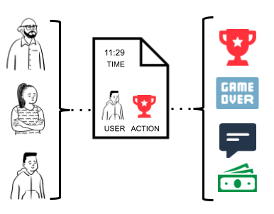
These events describe when users win, when they lose, when they buy things, when they they talk to each other. To make predictions we must train a model using examples composed of input features and target labels. Each example must be computed from the events we’re collecting.
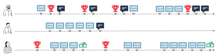
Visualizing events chronologically allows us to understand the context of each event, and the story of what’s happening.
-
The first player likes to brag about their victories
-
The game was too hard for the second player
-
The third player pays for upgrades when they get frustrated.
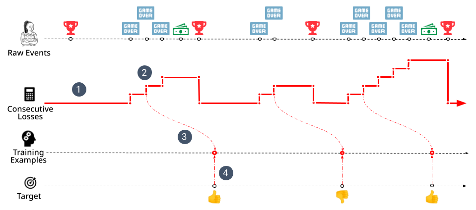
We’d like to capture this type of time-based insight as feature values we can use to train a model. We can do this by drawing the result of feature computations as a timeline showing how the feature’s value changes as each event is observed. This timeline allows us to “observe” the value of the feature at any point in time, giving us a framework for training real-time ML models:
-
Start with raw events and compute feature timelines
-
Observe features at the points in time a prediction would be made to build a training example
-
Move each example forward in time until the predicted outcome can be observed
-
Compute the correct target value and append it to the example
Implementing each of these four steps allows us to compute a set of training examples where each example captures the value of our model’s input features at a specific point in time as well as the model’s target label at a (potentially different) point in time.
Let’s explore how Kaskada allows us to implement this framework for our example problem. Kaskada treats events as rows in tables - we’ll focus on two tables describing the result of users playing our game, GameVictory and GameDefeat.
| time | entity | value |
|---|---|---|
|
|
|
|
|
|
|
|
|
|
|
|
|
|
|
| time | entity | value |
|---|---|---|
|
|
|
|
|
|
|
|
|
|
|
|
|
|
|
Step 1: Define features
We want to predict if a user will pay for an upgrade - step one is to compute features from events. As a first simple feature, we describe the amount of time a user as spent losing at the game - users who lose a lot are probably more likely to pay for upgrades.
let features = { (1)
loss_duration: sum(GameVictory.duration) } (2)| 1 | Construct a record containing a single field named loss_dur |
| 2 | Compute the sum of each victory event’s duration field |
| time | entity | result |
|---|---|---|
|
|
|
|
|
|
|
|
|
|
|
|
|
|
|
Notice that the result is a timeline describing the step function of how this feature has changed over time. We can “observe” the value of this step function at any time, regardless of the times at which the original events occurred.
Another thing to notice is that these results are automatically grouped by user. We didn’t have to explicitly group by user because tables in Kaskada specify an "entity" associated with each row.
Step 2: Define prediction times
The second step is to observe our feature at the times a prediction would have been made.
Let’s assume that the game designers want to offer an upgrade any time a user loses the game twice in a row.
We can construct a set of examples associated with this prediction time by observing our feature when the user loses twice in a row.
let features = {
  loss_duration: sum(GameVictory.duration) }

let examples = features (1)
| when(count(GameDefeat, window=since(GameVictory)) == 2) (2) (3)| 1 | The feature record we created previously |
| 2 | Build a sequence of operations using the pipe operator |
| 3 | You can think of this query as walking over our events chronologically, counting how many GameDefeat events have bene seen since the most recent GameVictory event |
| time | entity | result |
|---|---|---|
|
|
|
|
|
|
This query gives us a set of examples, each containing input features computed at the specific times we would like to make a prediction.
Step 3: Shift examples
The third step is to move each example to the time when the outcome we’re predicting can be observed. We want to give the user some time to see the upgrade offer, decide to accept it, and pay - let’s check to see if they accepted an hour after we make the offer.
let features = {
  loss_duration: sum(GameVictory.duration) }

let examples = features
  | when(count(GameDefeat, window=since(GameVictory)) == 2) (1)
| shift_by(hours(1)) (2)| 1 | The examples we created previously |
| 2 | Shift the results of the last step forward in time by one hour - visually you could imagine dragging the examples forward in the timeline by one hour |
| time | entity | result |
|---|---|---|
|
|
|
|
|
|
Our training examples have now moved to the point in time when the label we want to predict can be observed. Notice that the values in the time column are an hour later than the previous step.
Step 4: Label examples
The final step is to see if a purchase happened after the prediction was made. This will be our target value and we’ll add it to the records that currently contain our feature.
let features = {
  loss_duration: sum(GameVictory.duration),
  purchase_count: count(Purchase) }   (1)

let example = features
  | when(count(GameDefeat, window=since(GameVictory)) == 2)
  | shift_by(hours(1))

let target = count(Purchase) > example.purchase_count (2)

in extend(example, {target}) (3)| 1 | Capture purchase count as a feature |
| 2 | Compare purchase count at prediction and label time. |
| 3 | Append the target value to each example |
| time | entity | result |
|---|---|---|
|
|
|
|
|
|
We’re done! The result of this query is a training dataset ready to be used as input to a model algorithm. To review the process so far:
-
We computed the time spent in loosing games from the events we collected
-
We generated training examples each time the a user lost twice in a row
-
We shifted those examples forward in time one hour
-
Finally, we computed the target value by checking for purchases since the prediction was made.